 . A clique potential
depends on the type c (size, shape and possibly orientation) of the
clique and the local configuration
  . For
cliques containing more than one site (
 ), the MLL clique
potentials are defined by
The auto-logistic model can be generalized to multi-level logistic
(MLL) model [Elliott et al. 1984 ; Derin and Cole 1986 ; Derin and Elliott 1987], also called Strauss
process
[Strauss 1977] and generalized Ising model [Geman and Geman 1984]. There are M (>2) discrete
labels in the label set,  . A clique potential
depends on the type c (size, shape and possibly orientation) of the
clique and the local configuration
  . For
cliques containing more than one site (
 ), the MLL clique
potentials are defined by
where  is the potential for type-c cliques; for single site
cliques, they depends on the label assigned to the site
where  is the potential for label value I.
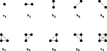
Fig.1.4 shows the clique types and the
associated parameters in the second order (8-neighbor) neighborhood
system.

Figure 1.4: Clique types and associated potential parameters for the
second order neighborhood system. Sites are shown in dots and
neighboring relationships in joining lines.
Assume that an MLL model is of second-order as in
(1.37), so that only  (for single-site
cliques) and
  (for pair-site cliques) parameters are non-zero.
The potential function for pair-wise cliques is written as
where  is the
  parameter for type-c cliques and
 is set of pair-site cliques. For the 4-neighborhood system,
there are four types of pair-wise cliques ( cf.
Fig.1.4) and so there may be four different
 's. When the model is isotropic all the four take the same
value. Owing to its simplicity, the pair-wise MLL model
(1.54) has been widely used for modeling regions and
textures
[Elliott et al. 1984 ; Geman and Geman 1984 ; Derin and Cole 1986 ; Derin and Elliott 1987 ; Murray and Buxton 1987 ; Lakshmanan and Derin 1989 ; Won and Derin 1992].
When the MLL model is isotropic, it depicts blob-like regions. In this case, the conditional probability can be expressed as follows [Strauss 1977]

where  is the number of sites in
  which are labeled I.
It reduces to (1.40) when there are
only two labels, 0 and 1. In contrast, an anisotropic model tends to
generates texture-like patterns. See examples in
Section 2.4.